数据集简介
MNIST(Modified National Institute of Standards and Technology database)是机器学习领域最著名、最常用的入门级图像分类数据集之一。它包含了大量手写数字的灰度图片,任务目标是正确识别出每张图片中的数字(0-9)。
由于其规模适中、任务直观、识别难度不高,它常被用作验证新算法或教学演示的“标准测试平台”,被誉为机器学习领域的 “Hello World”。
数据内容与结构
- 类别:10类,分别对应数字 0 到 9。
- 图像格式:每张图片是固定大小的 28×28 像素 的灰度图像。
- 像素值:每个像素是一个0到255之间的整数,0代表白色(背景),255代表纯黑色(笔迹),中间值是不同程度的灰色。
- 数据量:数据集通常被分为两部分:
- 训练集:60,000 张 图片,用于训练模型。
- 测试集:10,000 张 图片,用于评估模型的最终性能。
数据示例
每个样本通常由一个特征向量(图像数据)和一个标签(真实数字)组成。
- 原始图像:可以看作一个 28行 x 28列 的矩阵。
- 常用扁平化处理:在输入到许多经典机器学习模型(如逻辑回归、全连接神经网络)时,会将这个矩阵“展平”成一个长度为 784 (28*28) 的一维向量。
- 标签:一个 0-9 的整数,或通常被处理成 One-Hot 编码(例如,数字5表示为
[0,0,0,0,0,1,0,0,0,0])。本例中,我们将在代码中把整数5做One-Hot编码处理
代码详解
导入数据集
本例中使用keras的数据集包(keras.datasets)中的mnist数据集的load_data()函数直接加载mnist数据,其中:x_train 为训练集手写图片;y_train 为训练集标签;x_test 为测试集手写图片;y_test 为测试集标签
import keras
from keras.datasets import mnist

################################
# 加载mnist数据集
# x_train 为训练集手写图片
# y_train 为训练集标签
# x_test  为测试集手写图片
# y_test  为测试集标签
################################
(x_train, y_train), (x_test, y_test) = mnist.load_data()
查看数据集中的数据结构
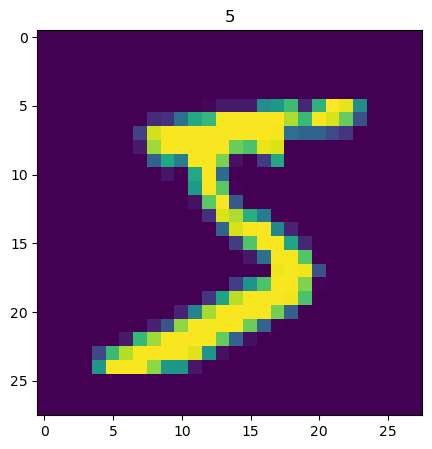
下面的代码显示训练集图片数据和标签数据的形状,显示训练集索引0(第一张手写图片)的图片和标签所示数字“5”
# 显示训练集x_train的形状 (60000, 28, 28)
# 为60000张,28*28像素的图片
print(x_train.shape)
# (60000, 28, 28)

# 显示训练集y_train的形状 (60000,)
# 为60000个标记手写图片所代表数字的数值
print(y_train.shape)
# (60000,)

# 这里显示训练集手写图片索引0的图片内容
import matplotlib
from matplotlib import pyplot as plt

# 训练集索引为0的图片
img1 = x_train[0]
# 训练集索引为0的标签
label1 = y_train[0]

# 这里显示训练集标签索引0的内容 5
print(f"label1: {label1}")
# label1: 5

print(img1.shape)
# (28, 28)

# 这里显示训练集数据索引0的图片
plt.figure(figsize=(5,5))
plt.imshow(img1)
plt.title(label1)
plt.show()
以下是输出:
(60000, 28, 28)
(60000,)
label1: 5
(28, 28)
把分类训练标签转换为分类数组
from keras.utils import to_categorical
#分类训练标签转换为分类数组,
y_train_format = to_categorical(y_train)
#分类数组0(y_train_format[0])中的索引5的值为1,表示分类数组0的手写图片的标签是5
print(y_train_format[0])
# [0. 0. 0. 0. 0. 1. 0. 0. 0. 0.]
以下是输出:
[0. 0. 0. 0. 0. 1. 0. 0. 0. 0.]
把28*28手写图片的二维点阵拍平为784长度的一维度数组
################################################################
# 我们把28*28手写图片的二维点阵拍平为784长度的一维度数组 x_train_format
# feature_size = 28 * 28,即784
################################################################
feature_size = (img1.shape[0] * img1.shape[1])
print(feature_size)
# 784

# 把x_train数据(60000*28*28),拍平为(60000*784)
x_train_format = x_train.reshape(x_train.shape[0], feature_size)
print(x_train_format.shape)
# (60000, 784)
以下是输出:
784
(60000, 784)
归一化图片数据
########################################
# 归一化x_train_format,使其值在0-1之间
# 灰度图片的每个点的值在0-255之间
# 归一化后的训练集为x_train_normal
########################################
x_train_normal = x_train_format / 255
构建多层神经网络(mlp)模型
from keras.models import Sequential
from keras.layers import Dense, ReLU, Input

#####################################
# 构建多层神经网络(mlp)模型
#####################################

# 构建空的模型容器
model = Sequential()

# 构建输入层,输入数据的形状为(feature_size,),即(384,)
model.add(Input(shape=(feature_size,)))

####################################################################
# 构建神经网络层(共3层)
# units 表示该层所包含的神经单元数,
# activation 表示该层使用的激活函数,这里使用的是 relu,其它常见的还有 sigmoid
####################################################################
dense1 = Dense(units=392, activation='relu')
dense2 = Dense(units=392, activation='relu')
#第三个神经网络层,含10个神经单元,使用softmax激活函数(用于多分类)
dense3 = Dense(units=10, activation='softmax')

#在模型中添加神经网络层
model.add(dense1)
#也可以单独增加每层的激活函数
#model.add(LeakyReLU(alpha=0.1))
model.add(dense2)
model.add(dense3)

# 显示神经网络模型的摘要
model.summary()
以下是输出:
Model: "sequential"
| Layer (type) | Output Shape | Param # |
| dense (Dense) | None, 392) | 307,720 |
| dense_1 (Dense) | (None, 392) | 154,056 |
| dense_2 (Dense) | (None, 10) | 3,930 |
Total params: 465,706 (1.78 MB)
Trainable params: 465,706 (1.78 MB)
Non-trainable params: 0 (0.00 B)
训练模型
# 设置模型的损失函数 loss为多分类交叉熵损失函数 和 优化器 optimizer为adam, 度量metrics 准确率accuracy,并编译模型
model.compile(loss='categorical_crossentropy', optimizer='adam', metrics=['accuracy'])
# 训练模型,输入优化过的训练集x_train_normal和训练集标签y_train_format,训练的迭代次数epochs为10次,训练的机构返回到history变量
history=model.fit(x_train_normal, y_train_format, epochs=10)
以下是输出
Epoch 1/10
1875/1875 ━━━━━━━━━━━━━━━━━━━━ 4s 545us/step - accuracy: 0.9038 - loss: 0.3224
Epoch 2/10
1875/1875 ━━━━━━━━━━━━━━━━━━━━ 1s 539us/step - accuracy: 0.9744 - loss: 0.0800
Epoch 3/10
1875/1875 ━━━━━━━━━━━━━━━━━━━━ 1s 562us/step - accuracy: 0.9828 - loss: 0.0515
Epoch 4/10
1875/1875 ━━━━━━━━━━━━━━━━━━━━ 1s 560us/step - accuracy: 0.9876 - loss: 0.0379
Epoch 5/10
1875/1875 ━━━━━━━━━━━━━━━━━━━━ 1s 550us/step - accuracy: 0.9901 - loss: 0.0306
Epoch 6/10
1875/1875 ━━━━━━━━━━━━━━━━━━━━ 1s 570us/step - accuracy: 0.9919 - loss: 0.0258
Epoch 7/10
1875/1875 ━━━━━━━━━━━━━━━━━━━━ 1s 584us/step - accuracy: 0.9925 - loss: 0.0227
Epoch 8/10
1875/1875 ━━━━━━━━━━━━━━━━━━━━ 1s 540us/step - accuracy: 0.9929 - loss: 0.0236
Epoch 9/10
1875/1875 ━━━━━━━━━━━━━━━━━━━━ 1s 543us/step - accuracy: 0.9941 - loss: 0.0183
Epoch 10/10
1875/1875 ━━━━━━━━━━━━━━━━━━━━ 1s 558us/step - accuracy: 0.9949 - loss: 0.0152
训练好的模型使用训练集的数据进行预测
import numpy as np
# 训练好的模型使用训练集的数据进行预测,预测结果放在y_train_predict_arr数组
y_train_predict_arr = model.predict(x_train_normal)
# 显示预测结果的形状
print(y_train_predict_arr.shape)
# (60000, 10)

# 显示预测结果索引0的内容
print(y_train_predict_arr[0])
# 数组的索引表示是数字的0-9,索引数同预测数字,数组里的内容是该索引(预测数字)的概率
# [0.0000000e+00 1.4491818e-36 1.8990632e-31 1.0056755e-18 0.0000000e+00 1.0000000e+00 5.7439224e-42 4.3064774e-39 2.1630945e-26 5.1030418e-23]

# 使用numpy的argmax函数找出预测概率最大的数组索引
y_train_predict=np.argmax(y_train_predict_arr,axis=1)
print(y_train_predict.shape)
# (60000,)
print(y_train_predict)
# [5 0 4 ... 5 6 8]
print(y_train_predict[0])
# 5

from sklearn.metrics import accuracy_score
# 计算训练集预测准确率
accuracy_train = accuracy_score(y_train, y_train_predict)
print(f'accuracy_train: {accuracy_train}')
# accuracy_train: 0.9979666666666667
以下是输出
(60000, 10)
[0.0000000e+00 1.4491818e-36 1.8990632e-31 1.0056755e-18 0.0000000e+00
 1.0000000e+00 5.7439224e-42 4.3064774e-39 2.1630945e-26 5.1030418e-23]
(60000,)
[5 0 4 ... 5 6 8]
5
accuracy_train: 0.9979666666666667
训练好的模型使用测试集的数据进行预测
# 同样拍平x_test
x_test_format = x_test.reshape(x_test.shape[0], feature_size)
# 同样,归一化 x_test_format
# 归一化后的测试集为x_test_normal
x_test_normal = x_test_format / 255
# 模型预测测试集的数据
y_test_predict_arr = model.predict(x_test_normal)
# 使用numpy的argmax函数找出预测概率最大的数组索引
y_test_predict=np.argmax(y_test_predict_arr,axis=1)
# 显示测试集预测数组的形状
print(y_test_predict_arr.shape)
# 显示测试集标签数组索引0的内容
print(y_test_predict_arr[0])
# 显示测试集预测的形状
print(y_test_predict.shape)
print(y_test_predict)
# 显示测试集索引0和测试集预测索引0的内容
print(y_test[0])
print(y_test_predict[0])
from sklearn.metrics import accuracy_score
# 计算测试集预测准确率
accuracy_test = accuracy_score(y_test, y_test_predict)
print(f'accuracy_test: {accuracy_test}')
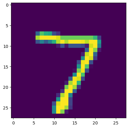
#显示测试集索引0的手写图片
img2 = x_test[0]
plt.figure(figsize=(5,5))
plt.imshow(img2)
plt.title(y_test_predict[0])
plt.show()
以下是输出
(10000, 10)
[3.7762964e-21 6.7931474e-19 5.9861794e-19 1.5149165e-21 2.3098683e-19
 5.6496597e-20 1.9527761e-27 1.0000000e+00 3.3848730e-19 5.9899928e-12]
(10000,)
[7 2 1 ... 4 5 6]
7
7
accuracy_test: 0.9824
查看指标变化
# 查看记录的指标名称,这里只有损失函数的变化的内容
print(history.history.keys())
# dict_keys(['accuracy', 'loss'])
# 显示准确率的变化
train_accuracy = history.history['accuracy']
print('train accuracy:')
print(train_accuracy)
# train accuracy:
# [0.9434166550636292, 0.9745333194732666, 0.9827666878700256, 0.9855999946594238, 0.9888499975204468, 0.9908666610717773, 0.9922833442687988, 0.9935666918754578, 0.9941333532333374, 0.9946333169937134]
# 显示损失函数变化
train_loss = history.history['loss']
print('train loss:')
print(train_loss)
# train loss:
# [0.019357334822416306, 0.014592494815587997, 0.016059745103120804, 0.014683437533676624, 0.013457028195261955, 0.013609101064503193, 0.014695452526211739, 0.012420445680618286, 0.013429272919893265, 0.010530633851885796]
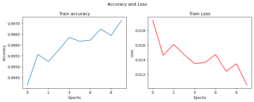
# 用图表显示准确率和损失函数的变化
fig, (ax1, ax2) = plt.subplots(1, 2, figsize=(10, 4))
ax1.plot(history.history['accuracy'])
ax1.set_title('Train accuracy')
ax1.set_xlabel('Epochs')
ax1.set_ylabel('Accuracy')
ax2.plot(history.history['loss'],'r')
ax2.set_title('Train Loss')
ax2.set_xlabel('Epochs')
ax2.set_ylabel('Loss')
fig.suptitle('Accuracy and Loss')
plt.tight_layout() # 自动调整子图参数,避免重叠
plt.show()
以下是输出
[0.9434166550636292, 0.9745333194732666, 0.9827666878700256, 0.9855999946594238, 0.9888499975204468, 0.9908666610717773, 0.9922833442687988, 0.9935666918754578,  0.9941333532333374, 0.9946333169937134]

[0.019357334822416306, 0.014592494815587997, 0.016059745103120804, 0.014683437533676624, 0.013457028195261955, 0.013609101064503193, 0.014695452526211739, 0.012420445680618286, 0.013429272919893265, 0.010530633851885796]
完整python代码
import keras
from keras.datasets import mnist

################################
# 加载mnist数据集
# x_train 为训练集手写图片
# y_train 为训练集标签
# x_test  为测试集手写图片
# y_test  为测试集标签
################################
(x_train, y_train), (x_test, y_test) = mnist.load_data()

# 显示训练集x_train的形状 (60000, 28, 28)
# 为60000张,28*28像素的图片
print(x_train.shape)
# (60000, 28, 28)

# 显示训练集y_train的形状 (60000,)
# 为60000个标记手写图片所代表数字的数值
print(y_train.shape)
# (60000,)

# 这里显示训练集手写图片索引0的图片内容
import matplotlib
from matplotlib import pyplot as plt

# 训练集索引为0的图片
img1 = x_train[0]
# 训练集索引为0的标签
label1 = y_train[0]

# 这里显示训练集标签索引0的内容 5
print(f"label1: {label1}")
# label1: 5

print(img1.shape)
# (28, 28)

# 这里显示训练集数据索引0的图片
plt.figure(figsize=(5,5))
plt.imshow(img1)
plt.title(label1)
plt.show()

from keras.utils import to_categorical
#分类训练标签转换为分类数组,
y_train_format = to_categorical(y_train)
#分类数组0(y_train_format[0])中的索引5的值为1,表示分类数组0的手写图片的标签是5
print(y_train_format[0])
# [0. 0. 0. 0. 0. 1. 0. 0. 0. 0.]

################################################################
# 我们把28*28手写图片的二维点阵拍平为784长度的一维度数组 x_train_format
# feature_size = 28 * 28,即784
################################################################
feature_size = (img1.shape[0] * img1.shape[1])
print(feature_size)
# 784

# 把x_train数据(60000*28*28),拍平为(60000*784)
x_train_format = x_train.reshape(x_train.shape[0], feature_size)
print(x_train_format.shape)
# (60000, 784)

########################################
# 归一化x_train_format,使其值在0-1之间
# 灰度图片的每个点的值在0-255之间
# 归一化后的训练集为x_train_normal
########################################
x_train_normal = x_train_format / 255

from keras.models import Sequential
from keras.layers import Dense, ReLU, Input

#####################################
# 构建多层神经网络(mlp)模型
#####################################

# 构建空的模型容器
model = Sequential()

# 构建输入层,输入数据的形状为(feature_size,),即(384,)
model.add(Input(shape=(feature_size,)))

####################################################################
# 构建神经网络层(共3层)
# units 表示该层所包含的神经单元数,
# activation 表示该层使用的激活函数,这里使用的是 relu,其它常见的还有 sigmoid
####################################################################
dense1 = Dense(units=392, activation='relu')
dense2 = Dense(units=392, activation='relu')
#第三个神经网络层,含10个神经单元,使用softmax激活函数(用于多分类)
dense3 = Dense(units=10, activation='softmax')

#在模型中添加神经网络层
model.add(dense1)
#也可以单独增加每层的激活函数
#model.add(LeakyReLU(alpha=0.1))
model.add(dense2)
model.add(dense3)

# 显示神经网络模型的摘要
model.summary()

# 设置模型的损失函数 loss为多分类交叉熵损失函数 和 优化器 optimizer为adam, 度量metrics 准确率accuracy,并编译模型
model.compile(loss='categorical_crossentropy', optimizer='adam', metrics=['accuracy'])
# 训练模型,输入优化过的训练集x_train_normal和训练集标签y_train_format,训练的迭代次数epochs为10次,训练的机构返回到history变量
history=model.fit(x_train_normal, y_train_format, epochs=10)

import numpy as np
# 训练好的模型使用训练集的数据进行预测,预测结果放在y_train_predict_arr数组
y_train_predict_arr = model.predict(x_train_normal)
# 显示预测结果的形状
print(y_train_predict_arr.shape)
# (60000, 10)

# 显示预测结果索引0的内容
print(y_train_predict_arr[0])
# 数组的索引表示是数字的0-9,索引数同预测数字,数组里的内容是该索引(预测数字)的概率
# [0.0000000e+00 1.4491818e-36 1.8990632e-31 1.0056755e-18 0.0000000e+00 1.0000000e+00 5.7439224e-42 4.3064774e-39 2.1630945e-26 5.1030418e-23]

# 使用numpy的argmax函数找出预测概率最大的数组索引
y_train_predict=np.argmax(y_train_predict_arr,axis=1)
print(y_train_predict.shape)
# (60000,)
print(y_train_predict)
# [5 0 4 ... 5 6 8]
print(y_train_predict[0])
# 5

from sklearn.metrics import accuracy_score
# 计算训练集预测准确率
accuracy_train = accuracy_score(y_train, y_train_predict)
print(f'accuracy_train: {accuracy_train}')
# accuracy_train: 0.9979666666666667

# 同样拍平x_test
x_test_format = x_test.reshape(x_test.shape[0], feature_size)

# 同样,归一化 x_test_format
# 归一化后的测试集为x_test_normal
x_test_normal = x_test_format / 255

# 模型预测测试集的数据
y_test_predict_arr = model.predict(x_test_normal)
# 使用numpy的argmax函数找出预测概率最大的数组索引
y_test_predict=np.argmax(y_test_predict_arr,axis=1)

# 显示测试集预测数组的形状
print(y_test_predict_arr.shape)
# 显示测试集标签数组索引0的内容
print(y_test_predict_arr[0])

# 显示测试集预测的形状
print(y_test_predict.shape)
print(y_test_predict)
# 显示测试集索引0和测试集预测索引0的内容
print(y_test[0])
print(y_test_predict[0])


from sklearn.metrics import accuracy_score
# 计算测试集预测准确率
accuracy_test = accuracy_score(y_test, y_test_predict)
print(f'accuracy_test: {accuracy_test}')

#显示测试集索引0的手写图片
img2 = x_test[0]
plt.figure(figsize=(5,5))
plt.imshow(img2)
plt.title(y_test_predict[0])
plt.show()

# 查看记录的指标名称,这里只有损失函数的变化的内容
print(history.history.keys())
# dict_keys(['accuracy', 'loss'])

# 显示准确率的变化
train_accuracy = history.history['accuracy']
print('train accuracy:')
print(train_accuracy)
# train accuracy:
# [0.9434166550636292, 0.9745333194732666, 0.9827666878700256, 0.9855999946594238, 0.9888499975204468, 0.9908666610717773, 0.9922833442687988, 0.9935666918754578,  0.9941333532333374, 0.9946333169937134]

# 显示损失函数变化
train_loss = history.history['loss']
print('train loss:')
print(train_loss)
# train loss:
# [0.019357334822416306, 0.014592494815587997, 0.016059745103120804, 0.014683437533676624, 0.013457028195261955, 0.013609101064503193, 0.014695452526211739, 0.012420445680618286, 0.013429272919893265, 0.010530633851885796]

# 用图表显示准确率和损失函数的变化
fig, (ax1, ax2) = plt.subplots(1, 2, figsize=(10, 4))
ax1.plot(history.history['accuracy'])
ax1.set_title('Train accuracy')
ax1.set_xlabel('Epochs')
ax1.set_ylabel('Accuracy')

ax2.plot(history.history['loss'],'r')
ax2.set_title('Train Loss')
ax2.set_xlabel('Epochs')
ax2.set_ylabel('Loss')

fig.suptitle('Accuracy and Loss')

plt.tight_layout() # 自动调整子图参数,避免重叠
plt.show()