数据集简介
MNIST(Modified National Institute of Standards and Technology database)是机器学习领域最著名、最常用的入门级图像分类数据集之一。它包含了大量手写数字的灰度图片,任务目标是正确识别出每张图片中的数字(0-9)。
由于其规模适中、任务直观、识别难度不高,它常被用作验证新算法或教学演示的“标准测试平台”,被誉为机器学习领域的 “Hello World”。
数据内容与结构
- 类别:10类,分别对应数字 0 到 9。
- 图像格式:每张图片是固定大小的 28×28 像素 的灰度图像。
- 像素值:每个像素是一个0到255之间的整数,0代表白色(背景),255代表纯黑色(笔迹),中间值是不同程度的灰色。
- 数据量:数据集通常被分为两部分:
- 训练集:60,000 张 图片,用于训练模型。
- 测试集:10,000 张 图片,用于评估模型的最终性能。
数据示例
每个样本通常由一个特征向量(图像数据)和一个标签(真实数字)组成。
- 原始图像:可以看作一个 28行 x 28列 的矩阵。
- 常用扁平化处理:在输入到许多经典机器学习模型(如逻辑回归、全连接神经网络)时,会将这个矩阵“展平”成一个长度为 784 (28*28) 的一维向量。
- 标签:一个 0-9 的整数,或通常被处理成 One-Hot 编码(例如,数字5表示为
[0,0,0,0,0,1,0,0,0,0])。本例中,我们将在代码中把整数5做One-Hot编码处理
代码详解
导入数据集
本例中使用keras的数据集包(keras.datasets)中的mnist数据集的load_data()函数直接加载mnist数据,其中:x_train 为训练集手写图片;y_train 为训练集标签;x_test 为测试集手写图片;y_test 为测试集标签
import keras
from keras.datasets import mnist

################################
# 加载mnist数据集
# x_train 为训练集手写图片
# y_train 为训练集标签
# x_test  为测试集手写图片
# y_test  为测试集标签
################################
(x_train, y_train), (x_test, y_test) = mnist.load_data()
查看数据集中的数据结构
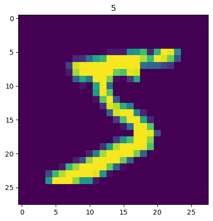
下面的代码显示训练集图片数据和标签数据的形状,显示训练集索引0(第一张手写图片)的图片和标签所示数字“5”
# 显示训练集x_train的形状 (60000, 28, 28)
# 为60000张,28*28像素的图片
print(x_train.shape)
# (60000, 28, 28)

# 显示训练集y_train的形状 (60000,)
# 为60000个标记手写图片所代表数字的数值
print(y_train.shape)
# (60000,)

# 这里显示训练集手写图片索引0的图片内容
import matplotlib
from matplotlib import pyplot as plt

# 训练集索引为0的图片
img1 = x_train[0]
# 训练集索引为0的标签
label1 = y_train[0]

# 这里显示训练集标签索引0的内容 5
print(f"label1: {label1}")
# label1: 5

print(img1.shape)
# (28, 28)

# 这里显示训练集数据索引0的图片
plt.figure(figsize=(5,5))
plt.imshow(img1)
plt.title(label1)
plt.show()
以下是输出:
(60000, 28, 28)
(60000,)
label1: 5
(28, 28)
把分类训练标签转换为分类数组
from keras.utils import to_categorical
#分类训练标签转换为分类数组,
y_train_format = to_categorical(y_train)
#分类数组0(y_train_format[0])中的索引5的值为1,表示分类数组0的手写图片的标签是5
print(y_train_format[0])
# [0. 0. 0. 0. 0. 1. 0. 0. 0. 0.]
以下是输出:
[0. 0. 0. 0. 0. 1. 0. 0. 0. 0.]
训练数据增加一个维度
import numpy as np
#############################################
# VGG网络是设计用于处理彩色图像的,其标准输入格式是:
# (batch_size, height, width, channels)
# 对于RGB图像:channels = 3 (红、绿、蓝)
# 对于灰度图像:channels = 1
#############################################
x_train_format = np.expand_dims(x_train, axis=3)
print(f'shape of x_train_format is {x_train_format.shape}')
# shape of x_train_format is (60000, 28, 28, 1)
以下是输出:
shape of x_train_format is (60000, 28, 28, 1)
归一化图片数据
########################################
# 归一化x_train_format,使其值在0-1之间
# 灰度图片的每个点的值在0-255之间
# 归一化后的训练集为x_train_normal
########################################
x_train_normal = x_train_format / 255
构建卷积神经网络(CNN)模型
from keras.models import Sequential
from keras.layers import Dense,Conv2D, MaxPooling2D, Flatten

#####################################
# 构建卷积神经网络(cnn)模型
#####################################

# 构建空的模型容器
model = Sequential()

##################################################################################
# 构建卷积层
# Conv2D 是二维卷积层,主要用于处理二维数据,如图像数据。它对输入数据应用卷积操作,提取空间特征。
# Conv2D(
#    filters=32,           # 滤波器的数量(输出通道数)
#    kernel_size=3,        # 卷积核大小(3x3)
#    strides=(1, 1),       # 滑动步长
#    padding='valid',      # 'valid'(不填充)或 'same'(填充)
#    activation='relu',    # 激活函数
#    input_shape=(28, 28, 1)  # 只在第一层需要
# )
#
# 卷积层输出形状公式
# 不填充 (valid)
# output_size = (input_size - kernel_size) / stride + 1
#
# 填充 (same)
# output_size = input_size / stride  # 当stride=1时,输出尺寸=输入尺寸
##################################################################################
conv1 = Conv2D(filters=32, kernel_size=(3,3), input_shape = (28,28,1), activation = 'relu')

##################################################################################
# 构建池化层
# MaxPooling2D 是卷积神经网络中的最大池化层,主要用于下采样(降维)和特征提取。
# MaxPooling2D(
#    pool_size=(2, 2),    # 池化窗口大小
#    strides=None,        # 步长(默认等于pool_size)
#    padding='valid',     # 填充方式
#    data_format=None     # 数据格式
#)
# activation 表示该层使用的激活函数,这里使用的是 relu,其它常见的还有 sigmoid
##################################################################################
pool1 = MaxPooling2D(pool_size = (2,2));

conv2 = Conv2D(filters=32, kernel_size=(3,3), input_shape = (28,28,1), activation = 'relu')
pool2 = MaxPooling2D(pool_size = (2,2));

model.add(conv1)
model.add(pool1)

model.add(conv2)
model.add(pool2)

flatten = Flatten()
model.add(flatten)

dense1 = Dense(units=800, activation='relu')
dense2 = Dense(units=10, activation='sigmoid')

model.add(dense1)
model.add(dense2)
model.summary()
以下是输出:
Model: "sequential"
| Layer (type) | Output Shape | Param # |
| conv2d (Conv2D) | (None, 26, 26, 32) | 320 |
| max_pooling2d (MaxPooling2D) | (None, 13, 13, 32) | 0 |
| conv2d_1 (Conv2D) | (None, 11, 11, 32) | 9,248 |
| max_pooling2d_1 (MaxPooling2D) | (None, 5, 5, 32) | 0 |
| flatten (Flatten) | (None, 800) | 0 |
| dense (Dense) | (None, 800) | 640,800 |
| dense_1 (Dense) | (None, 10) | 8,010 |
Total params: 658,378 (2.51 MB)
Trainable params: 658,378 (2.51 MB)
Non-trainable params: 0 (0.00 B)
训练模型
# 设置模型的损失函数 loss为多分类交叉熵损失函数 和 优化器 optimizer为adam, 度量metrics 准确率accuracy,并编译模型
model.compile(loss='categorical_crossentropy', optimizer='adam', metrics=['accuracy'])
# 训练模型,输入优化过的训练集x_train_normal和训练集标签y_train_format,训练的迭代次数epochs为10次,训练的机构返回到history变量
history=model.fit(x_train_normal, y_train_format, epochs=10)
以下是输出:
Epoch 1/10
1875/1875 ━━━━━━━━━━━━━━━━━━━━ 4s 846us/step - accuracy: 0.9182 - loss: 0.2660
Epoch 2/10
1875/1875 ━━━━━━━━━━━━━━━━━━━━ 2s 838us/step - accuracy: 0.9863 - loss: 0.0420
Epoch 3/10
1875/1875 ━━━━━━━━━━━━━━━━━━━━ 2s 840us/step - accuracy: 0.9909 - loss: 0.0282
Epoch 4/10
1875/1875 ━━━━━━━━━━━━━━━━━━━━ 2s 833us/step - accuracy: 0.9943 - loss: 0.0176
Epoch 5/10
1875/1875 ━━━━━━━━━━━━━━━━━━━━ 2s 839us/step - accuracy: 0.9962 - loss: 0.0124
Epoch 6/10
1875/1875 ━━━━━━━━━━━━━━━━━━━━ 2s 836us/step - accuracy: 0.9971 - loss: 0.0094
Epoch 7/10
1875/1875 ━━━━━━━━━━━━━━━━━━━━ 2s 840us/step - accuracy: 0.9967 - loss: 0.0099
Epoch 8/10
1875/1875 ━━━━━━━━━━━━━━━━━━━━ 2s 842us/step - accuracy: 0.9978 - loss: 0.0066
Epoch 9/10
1875/1875 ━━━━━━━━━━━━━━━━━━━━ 2s 843us/step - accuracy: 0.9976 - loss: 0.0076
Epoch 10/10
1875/1875 ━━━━━━━━━━━━━━━━━━━━ 2s 841us/step - accuracy: 0.9977 - loss: 0.0067
1875/1875 ━━━━━━━━━━━━━━━━━━━━ 1s 449us/step
训练好的模型使用训练集的数据进行预测
import numpy as np
# 训练好的模型使用训练集的数据进行预测,预测结果放在y_train_predict_arr数组
y_train_predict_arr = model.predict(x_train_normal)
# 显示预测结果的形状
print(y_train_predict_arr.shape)
# (60000, 10)

# 显示预测结果索引0的内容
print(y_train_predict_arr[0])
# 数组的索引表示是数字的0-9,索引数同预测数字,数组里的内容是该索引(预测数字)的概率
# [1.5303665e-10 7.9280517e-06 9.7667774e-10 9.9296063e-01 4.9890009e-10
# 1.0000000e+00 1.9100059e-07 3.5476958e-06 5.8910555e-05 1.2096505e-02]

# 使用numpy的argmax函数找出预测概率最大的数组索引
y_train_predict=np.argmax(y_train_predict_arr,axis=1)
print(y_train_predict.shape)
# (60000,)
print(y_train_predict)
# [5 0 4 ... 5 6 8]
print(y_train_predict[0])
# 5

from sklearn.metrics import accuracy_score
# 计算训练集预测准确率
accuracy_train = accuracy_score(y_train, y_train_predict)
print(f'accuracy_train: {accuracy_train}')
# accuracy_train: 0.9993333333333333
以下是输出:
(60000, 10)
[1.5303665e-10 7.9280517e-06 9.7667774e-10 9.9296063e-01 4.9890009e-10
 1.0000000e+00 1.9100059e-07 3.5476958e-06 5.8910555e-05 1.2096505e-02]
(60000,)
[5 0 4 ... 5 6 8]
5
accuracy_train: 0.9993333333333333
训练好的模型使用测试集的数据进行预测
# 同理,给测试数据集增加一个维度,变为(10000, 28, 28, 1)
x_test_format = np.expand_dims(x_test, axis=3)
print(f'shape of x_test_format is {x_test_format.shape}')
# shape of x_test_format is (10000, 28, 28, 1)
# 归一化测试集数据
x_test_normal = x_test_format / 255
# 模型预测测试集的数据
y_test_predict_arr = model.predict(x_test_normal)
# 使用numpy的argmax函数找出预测概率最大的数组索引
y_test_predict=np.argmax(y_test_predict_arr,axis=1)
# 显示测试集预测数组的形状
print(y_test_predict_arr.shape)
# 60000, 10)
# 显示测试集标签数组索引0的内容
print(y_test_predict_arr[0])
# [1.5303665e-10 7.9280517e-06 9.7667774e-10 9.9296063e-01 4.9890009e-10
# 1.0000000e+00 1.9100059e-07 3.5476958e-06 5.8910555e-05 1.2096505e-02]
# 显示测试集预测的形状
print(y_test_predict.shape)
# (10000,)
print(y_test_predict)
# [7 2 1 ... 4 5 6]
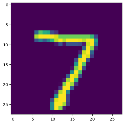
# 显示测试集索引0和测试集预测索引0的内容
print(y_test[0])
# 7
print(y_test_predict[0])
# 7
from sklearn.metrics import accuracy_score
# 计算测试集预测准确率
accuracy_test = accuracy_score(y_test, y_test_predict)
print(f'accuracy_test: {accuracy_test}')
# accuracy_test: 0.9927
#显示测试集索引0的手写图片
img2 = x_test[0]
plt.figure(figsize=(5,5))
plt.imshow(img2)
plt.title(y_test_predict[0])
plt.show()
以下是输出:
shape of x_test_format is (10000, 28, 28, 1)
(10000, 10)
[1.5303665e-10 7.9280517e-06 9.7667774e-10 9.9296063e-01 4.9890009e-10
 1.0000000e+00 1.9100059e-07 3.5476958e-06 5.8910555e-05 1.2096505e-02]
(10000,)
[7 2 1 ... 4 5 6]
7
7
accuracy_test: 0.9927
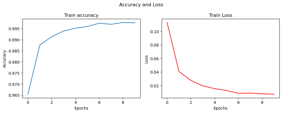
查看指标变化
# 查看记录的指标名称,这里只有损失函数的变化的内容
print(history.history.keys())
# dict_keys(['accuracy', 'loss'])

# 显示准确率的变化
train_accuracy = history.history['accuracy']
print('train accuracy:')
print(train_accuracy)
# train accuracy:
# [0.9660333395004272, 0.9873999953269958, 0.991599977016449, 0.9931666851043701, 0.995283305644989, 0.9962666630744934, 0.9965500235557556, 0.9972833395004272, 0.9975833296775818, 0.9978833198547363]

# 显示损失函数变化
train_loss = history.history['loss']
print('train loss:')
print(train_loss)
# train loss:
# [0.11468297243118286, 0.04034939780831337, 0.02613934315741062, 0.02069994993507862, 0.015140438452363014, 0.01182894129306078, 0.010227353312075138, 0.008562251925468445, 0.007741801906377077, 0.006608148105442524]

# 用图表显示准确率和损失函数的变化
fig, (ax1, ax2) = plt.subplots(1, 2, figsize=(10, 4))
ax1.plot(history.history['accuracy'])
ax1.set_title('Train accuracy')
ax1.set_xlabel('Epochs')
ax1.set_ylabel('Accuracy')

ax2.plot(history.history['loss'],'r')
ax2.set_title('Train Loss')
ax2.set_xlabel('Epochs')
ax2.set_ylabel('Loss')

fig.suptitle('Accuracy and Loss')

plt.tight_layout() # 自动调整子图参数,避免重叠
plt.show()
以下是输出:
[0.9660333395004272, 0.9873999953269958, 0.991599977016449, 0.9931666851043701, 0.995283305644989, 0.9962666630744934, 0.9965500235557556, 0.9972833395004272, 0.9975833296775818, 0.9978833198547363]

[0.11468297243118286, 0.04034939780831337, 0.02613934315741062, 0.02069994993507862, 0.015140438452363014, 0.01182894129306078, 0.010227353312075138, 0.008562251925468445, 0.007741801906377077, 0.006608148105442524]
完整python代码
import keras
from keras.datasets import mnist

################################
# 加载mnist数据集
# x_train 为训练集手写图片
# y_train 为训练集标签
# x_test  为测试集手写图片
# y_test  为测试集标签
################################
(x_train, y_train), (x_test, y_test) = mnist.load_data()

# 显示训练集x_train的形状 (60000, 28, 28)
# 为60000张,28*28像素的图片
print(x_train.shape)
# (60000, 28, 28)

# 显示训练集y_train的形状 (60000,)
# 为60000个标记手写图片所代表数字的数值
print(y_train.shape)
# (60000,)

# 这里显示训练集手写图片索引0的图片内容
import matplotlib
from matplotlib import pyplot as plt

# 训练集索引为0的图片
img1 = x_train[0]
# 训练集索引为0的标签
label1 = y_train[0]

# 这里显示训练集标签索引0的内容 5
print(f"label1: {label1}")
# label1: 5

print(img1.shape)
# (28, 28)

# 这里显示训练集数据索引0的图片
plt.figure(figsize=(5,5))
plt.imshow(img1)
plt.title(label1)
plt.show()

from keras.utils import to_categorical
#分类训练标签转换为分类数组,
y_train_format = to_categorical(y_train)
#分类数组0(y_train_format[0])中的索引5的值为1,表示分类数组0的手写图片的标签是5
print(y_train_format[0])
# [0. 0. 0. 0. 0. 1. 0. 0. 0. 0.]

import numpy as np
#############################################
# VGG网络是设计用于处理彩色图像的,其标准输入格式是:
# (batch_size, height, width, channels)
# 对于RGB图像:channels = 3 (红、绿、蓝)
# 对于灰度图像:channels = 1
#############################################
x_train_format = np.expand_dims(x_train, axis=3)
print(f'shape of x_train_format is {x_train_format.shape}')
# shape of x_train_format is (60000, 28, 28, 1)

########################################
# 归一化x_train_format,使其值在0-1之间
# 灰度图片的每个点的值在0-255之间
# 归一化后的训练集为x_train_normal
########################################
x_train_normal = x_train_format / 255

from keras.models import Sequential
from keras.layers import Dense,Conv2D, MaxPooling2D, Flatten

#####################################
# 构建卷积神经网络(cnn)模型
#####################################

# 构建空的模型容器
model = Sequential()

##################################################################################
# 构建卷积层
# Conv2D 是二维卷积层,主要用于处理二维数据,如图像数据。它对输入数据应用卷积操作,提取空间特征。
# Conv2D(
#    filters=32,           # 滤波器的数量(输出通道数)
#    kernel_size=3,        # 卷积核大小(3x3)
#    strides=(1, 1),       # 滑动步长
#    padding='valid',      # 'valid'(不填充)或 'same'(填充)
#    activation='relu',    # 激活函数
#    input_shape=(28, 28, 1)  # 只在第一层需要
# )
##################################################################################
conv1 = Conv2D(filters=32, kernel_size=(3,3), input_shape = (28,28,1), activation = 'relu')

##################################################################################
# 构建池化层
# MaxPooling2D 是卷积神经网络中的最大池化层,主要用于下采样(降维)和特征提取。
# MaxPooling2D(
#    pool_size=(2, 2),    # 池化窗口大小
#    strides=None,        # 步长(默认等于pool_size)
#    padding='valid',     # 填充方式
#    data_format=None     # 数据格式
#)
# activation 表示该层使用的激活函数,这里使用的是 relu,其它常见的还有 sigmoid
##################################################################################
pool1 = MaxPooling2D(pool_size = (2,2));

conv2 = Conv2D(filters=32, kernel_size=(3,3), activation = 'relu')
pool2 = MaxPooling2D(pool_size = (2,2));

model.add(conv1)
model.add(pool1)

model.add(conv2)
model.add(pool2)

flatten = Flatten()
model.add(flatten)

dense1 = Dense(units=800, activation='relu')
dense2 = Dense(units=10, activation='sigmoid')

model.add(dense1)
model.add(dense2)
model.summary()

# 设置模型的损失函数 loss为多分类交叉熵损失函数 和 优化器 optimizer为adam, 度量metrics 准确率accuracy,并编译模型
model.compile(loss='categorical_crossentropy', optimizer='adam', metrics=['accuracy'])
# 训练模型,输入优化过的训练集x_train_normal和训练集标签y_train_format,训练的迭代次数epochs为10次,训练的机构返回到history变量
history=model.fit(x_train_normal, y_train_format, epochs=10)

import numpy as np
# 训练好的模型使用训练集的数据进行预测,预测结果放在y_train_predict_arr数组
y_train_predict_arr = model.predict(x_train_normal)
# 显示预测结果的形状
print(y_train_predict_arr.shape)
# (60000, 10)

# 显示预测结果索引0的内容
print(y_train_predict_arr[0])
# 数组的索引表示是数字的0-9,索引数同预测数字,数组里的内容是该索引(预测数字)的概率
# [1.5303665e-10 7.9280517e-06 9.7667774e-10 9.9296063e-01 4.9890009e-10
# 1.0000000e+00 1.9100059e-07 3.5476958e-06 5.8910555e-05 1.2096505e-02]

# 使用numpy的argmax函数找出预测概率最大的数组索引
y_train_predict=np.argmax(y_train_predict_arr,axis=1)
print(y_train_predict.shape)
# (60000,)
print(y_train_predict)
# [5 0 4 ... 5 6 8]
print(y_train_predict[0])
# 5

from sklearn.metrics import accuracy_score
# 计算训练集预测准确率
accuracy_train = accuracy_score(y_train, y_train_predict)
print(f'accuracy_train: {accuracy_train}')
# accuracy_train: 0.9993333333333333

# 同理,给测试数据集增加一个维度,变为(10000, 28, 28, 1)
x_test_format = np.expand_dims(x_test, axis=3)
print(f'shape of x_test_format is {x_test_format.shape}')
# shape of x_test_format is (10000, 28, 28, 1)

# 归一化测试集数据
x_test_normal = x_test_format / 255

# 模型预测测试集的数据
y_test_predict_arr = model.predict(x_test_normal)
# 使用numpy的argmax函数找出预测概率最大的数组索引
y_test_predict=np.argmax(y_test_predict_arr,axis=1)

# 显示测试集预测数组的形状
print(y_test_predict_arr.shape)
# 60000, 10)

# 显示测试集标签数组索引0的内容
print(y_test_predict_arr[0])
# [1.5303665e-10 7.9280517e-06 9.7667774e-10 9.9296063e-01 4.9890009e-10
# 1.0000000e+00 1.9100059e-07 3.5476958e-06 5.8910555e-05 1.2096505e-02]

# 显示测试集预测的形状
print(y_test_predict.shape)
# (10000,)
print(y_test_predict)
# [7 2 1 ... 4 5 6]

# 显示测试集索引0和测试集预测索引0的内容
print(y_test[0])
# 7
print(y_test_predict[0])
# 7

from sklearn.metrics import accuracy_score
# 计算测试集预测准确率
accuracy_test = accuracy_score(y_test, y_test_predict)
print(f'accuracy_test: {accuracy_test}')
# accuracy_test: 0.9927

#显示测试集索引0的手写图片
img2 = x_test[0]
plt.figure(figsize=(5,5))
plt.imshow(img2)
plt.title(y_test_predict[0])
plt.show()

# 查看记录的指标名称,这里只有损失函数的变化的内容
print(history.history.keys())
# dict_keys(['accuracy', 'loss'])

# 显示准确率的变化
train_accuracy = history.history['accuracy']
print('train accuracy:')
print(train_accuracy)
# train accuracy:
# [0.9660333395004272, 0.9873999953269958, 0.991599977016449, 0.9931666851043701, 0.995283305644989, 0.9962666630744934, 0.9965500235557556, 0.9972833395004272, 0.9975833296775818, 0.9978833198547363]

# 显示损失函数变化
train_loss = history.history['loss']
print('train loss:')
print(train_loss)
# train loss:
# [0.11468297243118286, 0.04034939780831337, 0.02613934315741062, 0.02069994993507862, 0.015140438452363014, 0.01182894129306078, 0.010227353312075138, 0.008562251925468445, 0.007741801906377077, 0.006608148105442524]

# 用图表显示准确率和损失函数的变化
fig, (ax1, ax2) = plt.subplots(1, 2, figsize=(10, 4))
ax1.plot(history.history['accuracy'])
ax1.set_title('Train accuracy')
ax1.set_xlabel('Epochs')
ax1.set_ylabel('Accuracy')

ax2.plot(history.history['loss'],'r')
ax2.set_title('Train Loss')
ax2.set_xlabel('Epochs')
ax2.set_ylabel('Loss')

fig.suptitle('Accuracy and Loss')

plt.tight_layout() # 自动调整子图参数,避免重叠
plt.show()